고정 헤더 영역
상세 컨텐츠
본문
List of variables
dt = timestep
tau = decay time
spring constant = 1, mass = 1, omega = 1, period = 2 Pi,
nPeriod = 16, dt = 2 Pi/nPeriod, tau = 4 (2Pi)
Simulation tutorial
1) Generate new position
newP[p0_] :=
RandomReal[NormalDistribution[p0 Exp[-dt/tau], Sqrt[1 - Exp[-2 dt/tau]]]]
2) Verlet step simulation for a noisy harmonic oscillator

verletStep[p_, q_] := Module[{},
nextQ = q + p dt - q/2 dt^2;
nextP = p - (q + nextQ)/2 dt;
{nextP, nextQ}]
step[{p_, q_}] := verletStep[newP[p], q]
3) Verlet step simulation for a driven oscillator
verletStepDriven[p_, q_] := Module[{},
nextQ = q + p dt - q/2 dt^2 + a Cos[omega t]/2 dt^2;
nextP = p - (q + nextQ)/2 dt + (a Cos[omega t] + a Cos[omega (t + dt)])/ 2 dt;
t += dt;
{nextP, nextQ}]
stepDriven[{p_, q_}] := verletStepDriven[newP[p], q]
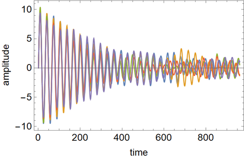
3) Examine reproducibility of momentum and position plot
nTraj = 5;
trajList = Table[NestList[step, {10., 0.}, 30 nPeriod], {nTraj}];
*position plot
ListPlot[Table[trajList[[i, All, 2]], {i, 1, nTraj}], Joined -> True, PlotRange -> All, Frame -> True, FrameLabel -> {"time", "amplitude"}]

*momentum plot
ListPlot[Table[trajList[[i, All, 1]], {i, 1, nTraj}], Joined -> True, PlotRange -> All, Frame -> True, FrameLabel -> {"time", "amplitude"}]
4) Driven response function
a = 0.2; t = 0.;
Table[omega = 0.85 + 0.05 n;
traj[n] = NestList[stepDriven, {0., 0.}, 30 nPeriod][[All, 2]], {n, 0, 6}];
ListPlot[Table[traj[n] + 10 (n - 3), {n, 0, 6}], Joined -> True,
PlotRange -> {-35, 35}, Frame -> True, FrameLabel -> {"time", "amplitude"}]

'Modeling > Mathematica' 카테고리의 다른 글
| Monte Carlo simulation of Leonnard-Jones fluid (0) | 2020.12.06 |
|---|---|
| Axial dispersion model (0) | 2020.12.06 |
| Ideal PFR (0) | 2020.12.06 |
| Ideal CSTR (0) | 2020.12.06 |
| Ideal Batch Reactor (0) | 2020.12.06 |


댓글 영역